Multipoint Methods for Improved Reservoir Models
Multipoint Methods for Improved Reservoir Models
The aim of this project is to develop new and improved methods for modelling geological facies by combining the efficiency of multipoint methods with the robustness and consistency of Markov random field methods. Develop software tools and test new methods on real cases and data.
Sub goals:
- Investigate advantages and limitations of the existing pixel based methods for modelling geological facies including multipoint methods (e.g. SNESIM) and Markov random field methods.
- Establish objective criteria to compare different methods beyond visual inspection. Connectivity and the prediction of fluid flow will be considered for this purpose.
- Get a deeper understanding of how multipoint methods work.
- Reduce artefacts in multipoint methods.
- Develop better ways of calibrating the methods to training images or other data.
- Develop practical methods for generating training images that appeal to a geologist.
- Investigate differences and similarities between multipoint methods and Markov random fields.
- Develop efficient software for pixel based facies models.
- Focus on efficient use of seismic data including time-lapse data (4D).
Multipoint methods
Multipoint methods are a set of pixel based simulation techniques. The term multipoint is used to stress that higher order statistics are used to capture the patterns seen in nature. This is in contrast to the variogram based techniques such as truncated Gaussian random fields and indicator kriging. In this sense, all methods we are investigating in this project are multipoint methods - including the Markov random field and Markov mesh models.
Simulating a discrete pixel based random field can be looked upon as a two step approach:
Estimation:
In the estimation step statistics from a training image (TI) is extracted. E.g. SNESIM stores the frequency of occurrence of all patterns in the TI within a predefined template. For Markov random fields a probability distribution is adapted to the TI using maximum likelihood estimation (MLE) or approximations to MLE.
Simulation:
Based on the estimates, a simulation algorithm will generate a sample that has the statistical properties of the TI. Furthermore, we want the simulated sample to be conditioned on data of different support.
The quality of the result depends on how well the relevant statistical properties of the TI are represented by the estimate and how the simulation algorithm perform. Presently, none of the considered approaches are perfect. They have different strengths and weaknesses.
Markov random fields
Markov random fields (MRF) are a class of probability distributions on a grid. The neighbourhood is the key concept for the Markov property: By definition the probability distribution for a particular grid cell value does only depend on the cell values within the neighbourhood of the grid cell. Assume for instance that we choose a 10 by 10 neighbourhood. For a binary problem (two facies types) there are 210 x 10 possibilities that we need to assign probabilities to. That is approximately 1030 possibilities! Consistency and assuming some symmetries will reduce this significantly but we are still left with a very rich model.
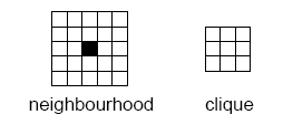
The probability model is often (without loss of generality) formulated in terms of potential functions of the grid values within a so called clique. The size of the maximal clique is approximately half the size of the neighbourhood in any direction. For a 10 by 10 neighbourhood the maximal clique is 6 by 6. This still leaves us with 1010 possible arguments for the potential functions.
Manually selecting a few potential functions is difficult since they have an unclear relation to the final simulation. Automated selection from a large set of possible potential functions is also problematic since it will rely on efficient estimation procedures. Maximum likelihood estimation is to tedious and pseudo-likelihood methods seems to fail.
Simulation of MRFs is done by Markov chain Monte Carlo using a Metropolis Hastings algorithm. These are iterative algorithms that in theory converge to the exact probability distribution. However, they might need many iterations for convergence so they are often to slow in practical applications. Conditioning on data is usually quite simple in these algorithms.
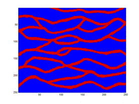
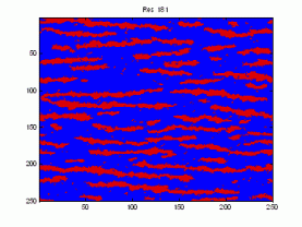
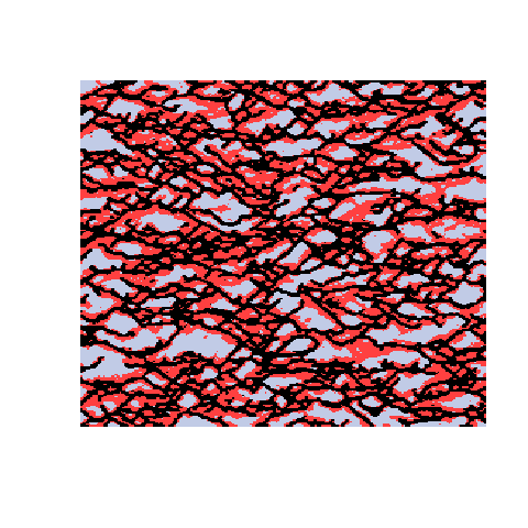
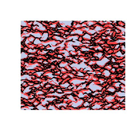
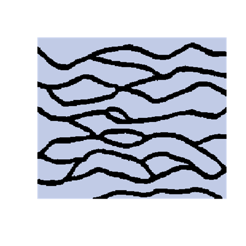
Here is a sample demonstrating that we are presently unable to replicate the patterns in the training image (left). The figure to the right is the result after 9050 iterations using potential functions including 3 point interactions.
Current work on Markov random fields are:
- Define and try maximum pseudo-block-likelihood estimation. Maximum likelihood estimation is the reference.
- Multi grid MRFs.
- Metropolis Hastings block proposals for conditional simulation.
Markov mesh models
Markov mesh models use an unsymmetrical neighbourhood. That makes both estimation and simulation a lot easier and faster. In particular simulation can be done sequentially and there is no need for iterations. The unsymmetrical neighbourhood introduces some skewness into the results but this can be counteracted by using two neighbourhoods - one for each direction.
The estimation part can be done successfully with MLE on a potentially large neighbourhood with higher order interactions. The simulation algorithm goes sequentially along the grid, line by line. The probabilities will only depend on the previously simulated values in the neighbourhood. The simulation is very fast.
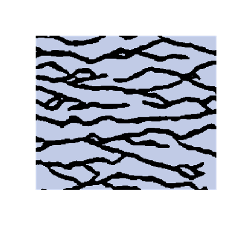
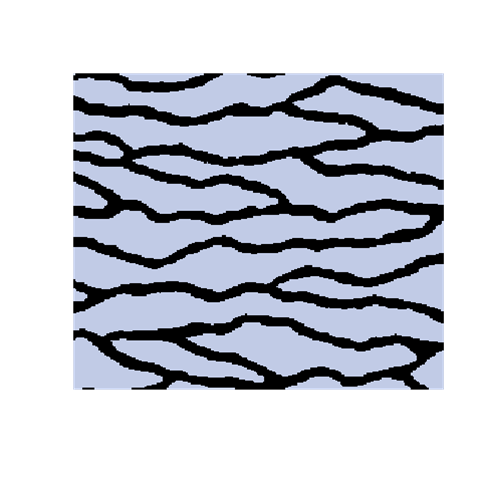
Here is an example with 3 facies types. The figures show the training image (left), a sample obtained using a Markov mesh model (middle), and a sample made by SNESIM (right). The simulated samples have a lot in common with the training image but they are generally more rugged.
The biggest challenge for the Markov mesh model is conditional simulation. Since the simulation algorithm only looks behind on previously simulated locations, data coming up in front are not accounted for properly.
Current work on Markov mesh models are:
- Conditioning to well data using kriging, extensions of existing method.
- Conditioning to well data using Markov random field iterations, global or local
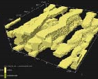
- Test on 3D training image. Case study based on North Sea data.
- Condition to seismic data.
- Local update. The current MMM implementation supports re-simulation of subparts of the grid. This mechanism can be used to re-simulate areas close to a newly introduced well. Semi-automatic ways of removing previously simulated parts of the grid must be implemented.
- Using Vines to construct the model directly from the TI.
SNESIM
Single Normal Equation Simulation (SNESIM) is the most well known and widely used multipoint simulation technique. A free version is available in S-GeMS. SNESIM is based on a simple idea:
- Count all pattern frequencies found in the training image.
-
Draw a random path through all grid cells in the simulation grid. Follow the random path sequentially and at each cell:
- Draw the current cell value according to the pattern frequencies found in the training image that match previously simulated cells.
- Store the drawn cell value and proceed to the next cell in the random path.
Note that the previously simulated cells may only cover very few cells so just small fragments of the training image are considered initially. Also note that the training image has limited size so it is common to ignore cells at distances beyond a predefined template.
Contrary to the two Markov approaches, the estimation step boils down to counting pattern frequencies. No probabilistic model is fitted to the training image. This purely empirical approach is commonly used in statistics when there is abundance of uncorrupted data. This simplifies the estimation step tremendously but makes the approach vulnerable to small training images.
The biggest challenge in the SNESIM approach is the simulation step. It looks simple and straight forward but there is a fundamental problem that needs to be dealt with: As the sequential simulation proceed along the random path, we look up the pattern frequencies in the training image. However, we only count patterns that match what has been drawn in the past and not what might be drawn in the future. In principal we should consider all possible future draws and compare them to the training image as well. This amounts to calculate the marginal probabilities at the current cell given the previously drawn cells. This is not possible to do for any realistically sized problem. So what happens is that the simulation gets stuck into partial patterns that do not exist in the training image. To resolve this, a method called node dropping is introduced. It amounts to ignoring some of the previously simulated cell values so that matches with the training image can be found. The practical consequence is that the final samples contain artefacts such as isolated cell values or object shapes not found in the training image.
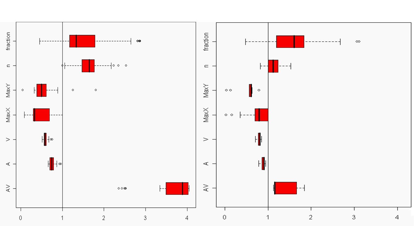
A modified SNESIM
The introduction of artefacts could be avoided by marginalizing the probabilities. However, this is computationally to expensive and maybe not a good solution. The training image will never include any acceptable pattern so some deviances should be allowed. We have tested an approach where we allow previously simulated cells values to be deleted so that they have to be re-drawn. Several criteria for selecting cells for re-simulation have been tested - some successful and some not. To the left are shown a training image (left), a sample using SNESIM (middle), and a sample using the modified SNESIM (right) where we re-draw some of the cell values. It is quite clear that the modification removes all the dead ends and that the sample to the right is visually closer to the training image. This is confirmed by the following picture showing box plots of statistics from 100 samples made by SNESIM (left) and the modified SNESIM (right). The vertical lines at 1 are the reference value obtained from the training image. The box plots show fraction of black cells, number of isolated objects, maximum vertical extension (of objects), maximum horizontal extension, area of objects, circumference of objects, and area/circumference at the bottom. So the statistics obtained from the modified algorithm are closer to the vertical lines at 1 showing that the modified SNESIM is better at replicating the training image properties.