- Rock Physics
- Rock Physics
Main | Mathematical Methods | CRAVA User Guide | Download
Inversion | Background model | Wavelet | Prior Correlations | Optimal Well Locations | Facies Probabilities | Rock Physics
The rock physics template model is very flexible, and requires an equally flexible implementation.
There are four main elements:
- Fluids.
- Solids.
- Rocks.
- Dry-rocks.
We handle these by a dual set of corresponding classes, the distribution classes and the sample classes. We have the set of DistributionFluid, DistributionSolid etc. base classes. These describe the prior distribution for different elements. From these, we can generate samples of the element. These samples are of base classes Fluid, Solid etc., and correspond directly to the Distributionclasses. Under the base classes, we have a set of derived classes, based on different rock physics models for mixing. These also exist on both distribution and sample version. Thus, the tree-like structure of a rock physics template model is mirrored here, with each prior distribution being built as a tree of Distribution... objects, and capable of generating a sample that is a similar tree of sample objects. The sample tree computes it properties as it is built, so the top level knows the resulting elastic parameters.
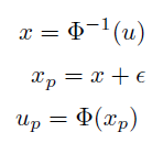
A feature of the rock physics implementation is that we can update a sample to generate a new sample. This new sample will be highly correlated with the initial sample. This is utilised to generate synthetic well data (for filtering), and when doing 4D modelling. In order to do this updating, each sample stores all the quantiles for the randomly drawn parameters in the sample. When updating a sample, each quantile u is perturbated to a quantile up as follows:

Here is normally distributed with expectation 0, and a variance based on the desired correlation. This sampling models the relation between the existing and new value as a Gaussian pair copula, with a given correlation parameter.

